6. Uniform Flow and Well#
The worksheet addresses the superposition of uniform and radial steady-state groundwater flow
in a homogeneous, confined aquifer of uniform thickness without recharge.
The radial flow component may represent an extraction or injection well.
Three travel time values representing isochrones can be selected by the user.
input parameters |
units |
remarks |
|---|---|---|
hydraulic conductivity |
m/s |
enter positive number |
effective porosity |
- |
enter number between 0 and 1 |
thickness |
mm/a |
enter positive number |
uniform velocity |
m/d |
enter number different from zero\(*\) |
pumping rate |
m³/d |
enter number different from zero\(**\) |
travel time |
d |
enter positive number |
\(*\) Positive or negative numbers correspond to uniform flow in parallel with or antiparallel to the x-axis, resp.
\(**\) Positive or negative numbers correspond to water extraction or injection, resp.
This tool can also be downloaded and run locally. For that download the uniform_flow_and_well.ipynb file from the book GitHub site, and execute the process in any editor (e.g., JUPYTER notebook, JUPYTER lab) that is able to read and execute this file-type.
The codes are licensed under CC by 4.0 (use anyways, but acknowledge the original work)
import streamlit as st
import matplotlib.pyplot as plt
from matplotlib import cm
import numpy as np
6.1. Streamline Isoline Calculation#
def case_well(X1_para,Y1_para,Q_para1,X2_para,Y2_para,Q_para2,K_para,Por_para,Qx_para ):


    H = 9.                                     # thickness [L]
    h0 = 9.5                                    # reference piezometric head [L]
    K = K_para * 5.e-5                          # hydraulic conductivity [L/T]
    por = Por_para                              # porosity []   old 0.25
    Qx0 = Qx_para * 1.e-10                      # baseflow in x-direction [L^2/T] was 1.e-6 before
    #Qy0 = Qy_para * 1.e-10                                    # baseflow in y-direction [L^2/T]
    Qy0 = 0
    # Wells
    xwell = np.array([X1_para, X2_para])        # x-coordinates well position [L] [99, 145]
    ywell = np.array([Y1_para, Y2_para])        # y-coordinates well position [L] [50, 78
    Qwell = np.array([Q_para1 * 1.e-4, Q_para2 * 1.e-4])   # pumping / recharge rates [L^3/T]
    R = [0.3, 0.2]                              # well radius [L]
    # Mesh
    xmin = 0           # minimum x-position of mesh [L]
    xmax = 200         # maximum x-position of mesh [L]
    ymin = 0           # minimum y-position of mesh [L]
    ymax = 200         # maximum y-position of mesh [L]


    # Reference point position in mesh
    iref = 1
    jref = 1

    # Graphical output options
    gsurfh = 1         # piezometric head surface plot
    gcontf = 10        # no. filled contour lines (=0: none)
    gquiv = 0          # arrow field plot
    gflowp_fit = 0     # flowpaths forward in time
    gflowp_bit = 0     # no. flowpaths backward in time (=0: none)
    gflowp_dot = 1     # flowpaths with dots indicating speed
    gstream = 10        # streamfunction plot            10


    #----------------------------------------execution-------------------------------
    xvec = np.linspace(xmin, xmax, 100)
    yvec = np.linspace(ymin, ymax, 100)
    [x, y] = np.meshgrid(xvec, yvec)                        # mesh
    phi = -Qx0 * x - Qy0 * y                                # baseflow potential
    psi = -Qx0 * y + Qy0 * x
    for i in range(0, xwell.size):                          # old version was: for i = 1:size(xwell,2)
        #r = np.sqrt((x - xwell[i]) * (x - xwell[i]) + (y - ywell[i]) * (y - ywell[i]))
        r = np.sqrt((x - xwell[i])**2 + (y - ywell[i])**2)
        phi = phi + (Qwell[i] / (2 * np.pi)) * np.log(r)    # potential
        psi = psi + (Qwell[i]/ (2 * np.pi)) * np.arctan2((y - ywell[i]), (x - xwell[i]))
    if h0 > H:
        phi0 = -phi[iref, jref] + K * H * h0 - 0.5 * K * H * H
    else:
        phi0 = -phi[iref, jref] + 0.5 * K * h0 * h0          # reference potential
    hc = 0.5 * H + (1 / K / H) * (phi + phi0)                     # head confined
    hu = np.sqrt((2 / K) * (phi + phi0))                      # head unconfined
    phicrit = phi0 + 0.5 * K * H * H                        # transition confined / unconfined
    confined = (phi >= phicrit)                         # confined / unconfined indicator
    h = confined * hc+ ~confined * hu                    # head

    [u,v] = np.gradient(-phi)                           # discharge vector
    Hh = confined * H + ~confined * h                   # aquifer depth
    u = u / Hh / (xvec[2] - xvec[1]) / por
    v = v / Hh / (yvec[2] - yvec[1]) / por
    #--------------------------------------graphical output--------------------
    if gsurfh:
        #plt.figure()
        fig, ax = plt.subplots(subplot_kw={"projection": "3d"})
        surf = ax.plot_surface(x, y, h,cmap=cm.coolwarm,linewidth=0,antialiased=True)                         # surface
        #plt.gca().zaxis.set_major_formatter(StrMethodFormatter('{x:,.4f}'))
        ax.set_xlabel('x [m]')
        ax.set_ylabel('y [m]')

        ax.set_zlabel('drawdown [m]')
        fig.colorbar(surf, shrink=.8, ax=[ax], location = "left") # ax=[ax], location='left' for left side

        #fig.colorbar(surf, shrink=0.5, aspect=10)
    if gcontf or gquiv or gflowp_fit or gflowp_bit or gflowp_dot or gstream:
        fig2, ax = plt.subplots()

        contour = plt.contour(x, y, h, gcontf, cmap=cm.Blues)
        contour2 = plt.contour(x, y, psi, gstream, colors=['#808080', '#808080', '#808080'], extend='both')

        ax.set_xlabel('x [m]')
        ax.set_ylabel('y [m]')

        contour.cmap.set_over('#808080')
        contour.cmap.set_under('blue')
        contour.changed()

        # Manually add color patches to the legend
        labels = ['Streamline', 'Potentialline']
        handles = [
            plt.Line2D([0], [0], color='#808080', lw=2),
            plt.Line2D([0], [0], color='blue', lw=2),
        ]

        plt.legend(handles, labels, loc='upper left')


    if gquiv:
        plt.quiver(x,y,v,u)                          # arrow field // quiver(x,y,u,v,'y')
    if gflowp_fit:                                      # flowpaths
        xstart = []
        ystart = []
        for i in range(100):
            if v[1,i] > 0:
                xstart = [xstart, xvec[i]]
                ystart = [ystart, yvec[1]]
            if v[99,i] < 0:
                xstart = [xstart, xvec[i]]
                ystart = [ystart, yvec[99]]
            if u[i,1] > 0:
                xstart = [xstart, xvec[1]]
                ystart = [ystart, yvec[i]]
            if u[i,99] < 0:
                xstart = [xstart, xvec[99]]
                ystart = [ystart, yvec[i]]

        h = plt.streamplot(x,y,u,v,)#,xstart,ystart)
        plt.streamplot(x,y,u,v,color='b')#,xstart,ystart)

    if gflowp_bit:
        for j in range(0, Qwell.size):
            if Qwell[j]>0:           # only for pumping wells
                xstart = xwell[j] + R[j]*np.cos(2*np.pi*np.array([1,1,gflowp_bit])/gflowp_bit)
                ystart = ywell[j] + R[j]*np.sin(2*np.pi*np.array([1,1,gflowp_bit])/gflowp_bit)
                seed_points = np.array([xstart,ystart])

                h = plt.streamplot(x,y,-u,-v,start_points=seed_points.T)


    plt.show()
#Testing the code
#case_well(X1_para=15,Y1_para=25,Q_para1=2,X2_para=30,Y2_para=40,Q_para2=1,K_para=2.1,Por_para=0.6,Qx_para=2 )
6.2. Enter Data using the Widgets below#
import ipywidgets as widgets
from IPython.display import display, clear_output, HTML

# Function to create and display widgets based on the number of wells selected
def create_widgets(num_wells):
    #print(num_wells)
    # Define the widgets
    style = {'description_width': 'initial'}
    if num_wells==2 :
        X1_para = widgets.FloatText(value=75, description='X Position Well 1',style=style)
        Y1_para = widgets.FloatText(value=100, description='Y Position Well 1',style=style)
        Q_para1 = widgets.FloatText(value=1, description='Pumping Rate Well 1',style=style)
        X2_para = widgets.FloatText(value=150, description='X Position Well 2',style=style)
        Y2_para = widgets.FloatText(value=100, description='Y Position Well 2',style=style)
        Q_para2 = widgets.FloatText(value=1, description='Pumping Rate Well 2',style=style)
        K_para = widgets.FloatText(value=6.3, description='Hydraulic Conductivity (K)',style=style)
        Por_para = widgets.FloatText(value=0.6, description='Porosity (ne)',style=style)
        Qx_para = widgets.FloatText(value=1, description='Baseflow Discharge (Qx)',style=style)

        # Function to be called on widget change
        def on_widget_change(change):
            clear_output(wait=True)
            hbox1 = widgets.HBox([X1_para, Y1_para, Q_para1])
            hbox2 = widgets.HBox([X2_para, Y2_para, Q_para2])
            hbox3 = widgets.HBox([K_para, Por_para, Qx_para])
            vbox = widgets.VBox([hbox1, hbox2, hbox3])
            display(vbox)
            case_well(
                X1_para.value, Y1_para.value, Q_para1.value,
                X2_para.value, Y2_para.value, Q_para2.value,
                K_para.value, Por_para.value, Qx_para.value
            )

        # Observe changes in the widgets
        X1_para.observe(on_widget_change, 'value')
        Y1_para.observe(on_widget_change, 'value')
        Q_para1.observe(on_widget_change, 'value')
        X2_para.observe(on_widget_change, 'value')
        Y2_para.observe(on_widget_change, 'value')
        Q_para2.observe(on_widget_change, 'value')
        K_para.observe(on_widget_change, 'value')
        Por_para.observe(on_widget_change, 'value')
        Qx_para.observe(on_widget_change, 'value')

        # Initial display
        on_widget_change(None)
    if num_wells==1 :
        X1_para = widgets.FloatText(value=75, description='X Position Well 1',style=style)
        Y1_para = widgets.FloatText(value=100,  description='Y Position well 1',style=style)
        Q_para1 = widgets.FloatText(value=1,  description='Pumping Rate Well 1',style=style)
        #X2_para = widgets.FloatText(value=150, description='X-well 2')
        #Y2_para = widgets.FloatText(value=100, description='Y-well 2')
        #Q_para2 = widgets.FloatText(value=1, description='Pumping 2')
        K_para = widgets.FloatText(value=6.3,description='Hydraulic Conductivity (K)',style=style)
        Por_para = widgets.FloatText(value=0.6, description='Porosity (ne)',style=style)
        Qx_para = widgets.FloatText(value=1, description='Baseflow Discharge (Qx)',style=style)

        # Function to be called on widget change
        def on_widget_change(change):
            clear_output(wait=True)
            hbox1 = widgets.HBox([X1_para, Y1_para, Q_para1])
            #hbox2 = widgets.HBox([X2_para, Y2_para, Q_para2])
            hbox3 = widgets.HBox([K_para, Por_para, Qx_para])
            vbox = widgets.VBox([hbox1, hbox3])
            X2_para=0
            Y2_para=0
            Q_para2=0
            display(vbox)
            case_well(
                X1_para.value, Y1_para.value, Q_para1.value,
                X2_para, Y2_para, Q_para2,
                K_para.value, Por_para.value, Qx_para.value
            )

        # Observe changes in the widgets
        X1_para.observe(on_widget_change, 'value')
        Y1_para.observe(on_widget_change, 'value')
        Q_para1.observe(on_widget_change, 'value')
        #X2_para.observe(on_widget_change, 'value')
        #Y2_para.observe(on_widget_change, 'value')
        #Q_para2.observe(on_widget_change, 'value')
        K_para.observe(on_widget_change, 'value')
        Por_para.observe(on_widget_change, 'value')
        Qx_para.observe(on_widget_change, 'value')

        # Initial display
        on_widget_change(None)

# Dropdown to select the number of wells
num_wells_dropdown = widgets.Dropdown(options=['Select',1, 2], description='Number of Wells')

# Function to be called on dropdown change
def on_dropdown_change(change):
    clear_output(wait=True)
    display(num_wells_dropdown)
    create_widgets(change.new)

# Observe changes in the dropdown
num_wells_dropdown.observe(on_dropdown_change, 'value')

# Display the dropdown
display(num_wells_dropdown)
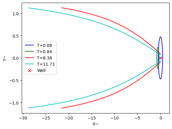
6.3. Isochrones and Capture Zones#
The following script is based on the publication On Using Simple Time-of-Travel Capture Zone Delineation Methods by Admir Ceric and Henk Haitjema This can be used to plot the capture zone of a well, given he time of travel.
import numpy as np
import matplotlib.pyplot as plt

def calculate_Lu(T):
    return T + np.log(T + np.e)

def calculate_y(T, x):
    Lu = calculate_Lu(T)
    return np.arctan(x / Lu)

def calculate_radius(T):
    return 1.161 * np.log(0.39 + T)

def calculate_eccentricity(T):
    return 0.00278 + (0.652 * T)

def calculate_radius_regular(T):
    return 1.6324 * np.sqrt(T)


def plotter(T_values) :

    # Define the range of T values
    #T_values = [0.05, 0.08, 0.1, 0.6, 0.9, 1.2, 3, 6]

    # Define a color palette for the lines
    colors = ['b', 'g', 'r', 'c', 'm', 'y', 'k', 'purple', 'orange', 'lime']

    # Loop through T values and plot accordingly
    for i, T in enumerate(T_values):
        color = colors[i % len(colors)]  # Cycle through colors if more than 10 T values

        if T <= 0.1:
            R = calculate_radius_regular(T)
            theta = np.linspace(0, 2*np.pi, 100)
            x = R * np.cos(theta)
            y = R * np.sin(theta)

            plt.plot(x, y, label=f'T={"{:.2f}".format(T)}', color=color)
        elif T <= 1:
            R = calculate_radius(T)
            d = calculate_eccentricity(T)

            theta = np.linspace(0, 2*np.pi, 100)
            x = R * np.cos(theta) + d
            y = R * np.sin(theta)
            x = -x

            plt.plot(x, y, label=f'T={"{:.2f}".format(T)}', color=color)
            #plt.scatter(0, 0, color='red', label='Upgradient Shift', marker='x')
        else:
            Lu = calculate_Lu(T)

            x = np.linspace(0, 2*Lu, 100)  # x~ from 0 to 2Lu
            y = np.linspace(0, 1, 100)
            x = -x
            y = calculate_y(T, x-1)

            plt.plot(x, y, label=f'T={"{:.2f}".format(T)}', color=color)
            plt.plot(x, -y, color=color)

    # Add legend and labels
    plt.scatter(0, 0, color='red', label='Well', marker='x')
    plt.legend()
    plt.xlabel('X~')
    plt.ylabel('Y~')

    # Display all the plots together at the end
    plt.show()
6.3.1. Enter Data using Widgets below#
# Create nine FloatText widgets
import math
import ipywidgets as widgets
from IPython.display import display, clear_output

def calculate_tdash(Qo,Q,H,n,T1,T2,T3,T4):
    T=[T1,T2,T3,T4]
    #print(T)
    Tdash=[]
    for t in T :
        Tdash.append((2 * math.pi * Qo**2 * t) / (n * H * Q))
    #print(Tdash)
    return(Tdash)


style = {'description_width': 'initial'}
widget1 = widgets.FloatText(value=2, description='Ambient Flow Qo [L2/T]',style=style)
widget2 = widgets.FloatText(value=3, description='Well Discharge Q [L3/T]',style=style)
widget3 = widgets.FloatText(value=20, description='Thickness Aquifier H [L]',style=style)
widget4 = widgets.FloatText(value=0.25, description='effective porosity',style=style)

widget5 = widgets.FloatText(value=0.05, description='time-of-travel [T]',style=style)
widget6 = widgets.FloatText(value=0.5, description='time-of-travel [T]',style=style)
widget7 = widgets.FloatText(value=5, description='time-of-travel [T]',style=style)
widget8 = widgets.FloatText(value=7, description='time-of-travel [T]',style=style)


# Function to be called on widget change
def on_widget_change(change):
    Tdash=[]
    clear_output(wait=True)
    # Create three HBox layouts to contain the widgets
    hbox1 = widgets.HBox([widget1, widget2])
    hbox2 = widgets.HBox([widget3, widget4])
    hbox3 = widgets.HBox([widget5, widget6, widget7,widget8])

    # Create a VBox layout to contain the three HBox layouts
    vbox = widgets.VBox([hbox1, hbox2, hbox3])

    # Display the VBox layout
    display(vbox)
    Tdash=calculate_tdash(widget1.value,widget2.value,widget3.value,widget4.value,widget5.value,widget6.value,widget7.value,widget8.value)
    plotter(Tdash)


widget1.observe(on_widget_change, 'value')
widget2.observe(on_widget_change, 'value')
widget3.observe(on_widget_change, 'value')
widget4.observe(on_widget_change, 'value')
widget5.observe(on_widget_change, 'value')
widget6.observe(on_widget_change, 'value')
widget7.observe(on_widget_change, 'value')
widget8.observe(on_widget_change, 'value')
on_widget_change(None)