Example 1: Basic Modelling with PyTracerLab

Here we show how to use the PyTracerLab package to perform the most basic standard application of lumped parameter models: calibrating parameter values (especially mean travel time of the travel time distribution) of the lumped parameter model from observations of tracer concentrations in an observation well.

import PyTracerLab.model as ism
import numpy as np
import matplotlib.pyplot as plt
from datetime import datetime

1. Load (Synthetic) Observation Data

See Example 4 on how this data is generated.

# load input series
# this would be the tracer concentration in precipitation or recharge in a
# practical problem
file_name = "example_input_series_1tracer.csv"
data = np.genfromtxt(
    file_name,
    delimiter=",",
    dtype=["<U7", float],
    encoding="utf-8",
    skip_header=1
)

timestamps = np.array([datetime.strptime(row[0], r"%Y-%m") for row in data])
input_series = np.array([float(row[1]) for row in data])

# load observation series
# this would be the measured tracer concentration in groudnwater in a
# practical problem
file_name = "example_observation_series_1tracer.csv"
data = np.genfromtxt(
    file_name,
    delimiter=",",
    dtype=["<U7", float],
    encoding="utf-8",
    skip_header=1
)

timestamps = np.array([datetime.strptime(row[0], r"%Y-%m") for row in data])
obs_series = np.array([float(row[1]) for row in data])

# load full system output series
# this would be the true tracer concentration in groudnwater in a practical
# problem; this is not available in practice
file_name = "example_output_series_1tracer.csv"
data = np.genfromtxt(
    file_name,
    delimiter=",",
    dtype=["<U7", float],
    encoding="utf-8",
    skip_header=1
)

timestamps = np.array([datetime.strptime(row[0], r"%Y-%m") for row in data])
output_series = np.array([float(row[1]) for row in data])

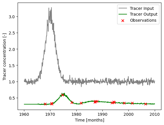
### plot input series, output series, and observations

# get observation timesteps
timesteps = [t.year + t.month / 12.0 for t in timestamps]

# create figure
fig, ax = plt.subplots(1, 1)
# plot input series
ax.plot(
    timesteps,
    input_series,
    label="Tracer Input",
    c="grey"
)
# plot output series
ax.plot(
    timesteps,
    output_series,
    label="Tracer Output",
    c="green"
)
# plot observations
ax.scatter(
    timesteps,
    obs_series,
    label="Observations",
    color="red",
    marker="x",
    zorder=10
)
ax.set_xlabel("Time [months]")
ax.set_ylabel("Tracer concentration [-]")
ax.legend()
plt.show()

2. Calibrate Model Parameters

t_half = 12.3 * 12.0
lambda_ = np.log(2.0) / t_half

### define model (use the same structure / units as the true model)
# time step is 1 month
m = ism.Model(
    dt=1.0,
    lambda_=lambda_,
    input_series=input_series,
    target_series=obs_series,
    steady_state_input=1., # this is the true value
    n_warmup_half_lives=10
)

# add an exponential-piston-flow unit
# define the initial model parameters for inference
epm_mtt_init = 12 * 1 # 1 year
epm_eta_init = 1.1
m.add_unit(
    ism.EPMUnit(mtt=epm_mtt_init, eta=epm_eta_init),
    fraction=.8, # 80 percent of the overall response; is the true value
    bounds=[(1.0, 12.0 * 50.), (1.0, 3.0)],
    prefix="epm"
)

# add a piston-flow unit
# define the true model parameters
pm_mtt_init = 12 * 1 # 1 year
m.add_unit(
    ism.PMUnit(mtt=pm_mtt_init),
    fraction=.2, # 20 percent of the overall response, is the true value
    bounds=[(1.0, 12.0 * 50.)],
    prefix="pm"
)

# create a solver
solver = ism.Solver(m)
# run DE
sol, sim = solver.differential_evolution(maxiter=10000, popsize=10)

# define true parameters
epm_mtt_true = 12 * 40 # 40 years
epm_eta_true = 1.5
pm_mtt_true = 12 * 5 # 5 years (faster than EPM)

# print solution
print("EPM MTT (true):", epm_mtt_true, "EPM MTT (cal):", sol["epm.mtt"])
print("EPM Eta (true):", epm_eta_true, "EPM Eta (cal):", sol["epm.eta"])
print("PM MTT (true):", pm_mtt_true, "PM MTT (cal):", sol["pm.mtt"])

EPM MTT (true): 480 EPM MTT (cal): 484.3422808609019
EPM Eta (true): 1.5 EPM Eta (cal): 1.4664123142091618
PM MTT (true): 60 PM MTT (cal): 60.49984389012326

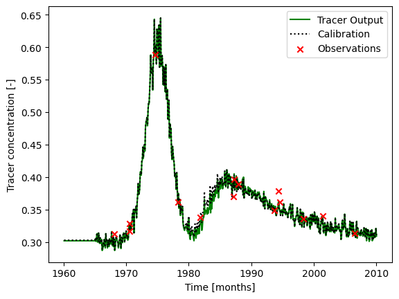
### plot input series, true output series, observations, and´
# calibrated output

# create figure
fig, ax = plt.subplots(1, 1)
# plot output series
ax.plot(
    timesteps,
    output_series,
    label="Tracer Output",
    c="green",
    zorder=0
)
# plot calibrated results
ax.plot(
    timesteps,
    sim,
    label="Calibration",
    c="black",
    alpha=1.,
    ls=":"
)

# plot observations
ax.scatter(
    timesteps,
    obs_series,
    label="Observations",
    color="red",
    marker="x",
    zorder=100000000
)
ax.set_xlabel("Time [months]")
ax.set_ylabel("Tracer concentration [-]")
ax.legend()
plt.show()