Example 6: Temporal Resolution Demonstration and Benchmark

Model simulations depend on the temporal resolution used. A model with monthly time steps of tracer input behaves differently than a model with yearly time steps. Here we demonstrate the differences and benchmark the use of the time step size parameter for the model (dt) to convert units.

import PyTracerLab.model as ism
import numpy as np
import matplotlib.pyplot as plt
from datetime import datetime

1. Load (Synthetic) Observation Data

See Example 4 on how this data is generated.

# load input series on monthly time steps
# this would be the tracer concentration in precipitation or recharge in a
# practical problem
file_name = "benchmark_input_monthly.csv"
data_m = np.genfromtxt(
    file_name,
    delimiter=",",
    dtype=["<U7", float],
    encoding="utf-8",
    skip_header=1
)

timestamps_m = np.array([datetime.strptime(row[0], r"%Y-%m") for row in data_m])
input_series_m = np.array([float(row[1]) for row in data_m])

# load input series on monthly time steps
# this would be the tracer concentration in precipitation or recharge in a
# practical problem
file_name = "benchmark_input_yearly.csv"
data_y = np.genfromtxt(
    file_name,
    delimiter=",",
    dtype=["<U7", float],
    encoding="utf-8",
    skip_header=1
)

timestamps_y = np.array([datetime.strptime(row[0], r"%Y") for row in data_y])
input_series_y = np.array([float(row[1]) for row in data_y])
# the monthly series has months as time units; we have to divide the yearly
# values by 12 to get the monthly values
input_series_y /= 12.

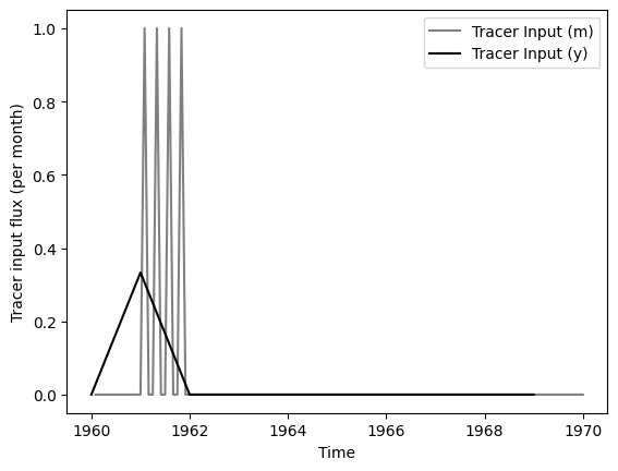
### plot input series, output series, and observations

# get observation timesteps
timesteps_m = [t.year + t.month / 12.0 for t in timestamps_m]
timesteps_y = [t.year for t in timestamps_y]

# create figure
fig, ax = plt.subplots(1, 1)
# plot input series monthly
ax.plot(
    timesteps_m,
    input_series_m,
    label="Tracer Input (m)",
    c="grey"
)
# plot input series yearly
ax.plot(
    timesteps_y,
    input_series_y,
    label="Tracer Input (y)",
    c="black"
)
ax.set_xlabel("Time")
ax.set_ylabel("Tracer input flux (per month)")
ax.legend()
plt.show()

2. Simulation

t_half = 12.3 * 12.0 # monthly half life
lambda_ = np.log(2.0) / t_half

### define model monthly
# time step is 1 month
m_m = ism.Model(
    dt=1.0,
    lambda_=lambda_,
    input_series=input_series_m,
    target_series=None,
    steady_state_input=0.,
    n_warmup_half_lives=10
)

# add an exponential unit
# define the initial model parameters
em_mtt_init = 12 * 1 # 1 year
m_m.add_unit(
    ism.EMUnit(mtt=em_mtt_init),
    fraction=1.,
    prefix="em"
)

### define model yearly
# time step is 1 month
m_y = ism.Model(
    dt=12., # 1 year is 12 months, so we have to adjust the time step
    lambda_=lambda_, # because we change the time step, we leave the lambda unchanged
    input_series=input_series_y,
    target_series=None,
    steady_state_input=0.,
    n_warmup_half_lives=10
)

# add an exponential unit
# define the initial model parameters
em_mtt_init = 12 * 1 # 1 year but in months again
m_y.add_unit(
    ism.EMUnit(mtt=em_mtt_init),
    fraction=1.,
    prefix="em"
)

# simulate with both models
sim_m = m_m.simulate()
sim_y = m_y.simulate()

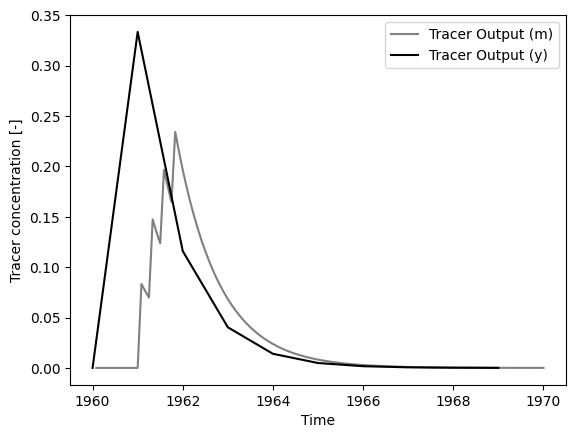
# plot output series
fig, ax = plt.subplots(1, 1)
ax.plot(
    timesteps_m,
    sim_m,
    label="Tracer Output (m)",
    c="grey"
)
ax.plot(
    timesteps_y,
    sim_y,
    label="Tracer Output (y)",
    c="black"
)
ax.set_xlabel("Time")
ax.set_ylabel("Tracer concentration [-]")
ax.legend()
plt.show()

test
test